Observations of Exoplanet Transits from Wallace Observatory: End of Summer Report
MIT Department of Earth Atmosphere and Planetary Science; MIT Department of Physics
(Dated: August 19, 2009)
1. SCIENTIFIC BACKGROUND
Scientists have, as of the beginning of August 2009, discovered over 350 planets around other stars. Of these extrasolar planets, about 60 are known to transit, or orbit in front of, the central star. The transiting planet will block a percentage of light from the star during the transit. The change in light flux from the star during transit varies between 2.8% for the deepest known transit and 0.3% for the shallowest. These transiting systems allow us to characterize physical properties of the planets, such as the ratio of its radius to that of its host star, to within a few percent.
The planetary system can also be characterized by a series of transit measurements of the same planet. If a second planet, in addition to the transiting planet, existed in the system, it would cause slight perturbations in the orbit of the transiting planet. By measuring the deviations from the expected transit time very precisely on a series of transits, a low-mass planet in the system could be detected. These kinds of detections are important in the search for earth-mass planets.
2. SUMMER WORK
Throughout this summer, I have been observing transiting planets from Wallace Observatory.
∗ Electronic address: cmorley@mit.edu
I have successfully observed five transits so far this summer. These summer observations will supply much of the data for my senior thesis project, as I am entering my senior year at MIT.
I started by learning to use the Mathematica code that the graduate student I was working with, Elisabeth Adams, had developed to predict when transits would occur. I created a calendar of the transits that would occur this summer and went to Wallace Observatory to observe them whenever a transit coincided with clear skies.
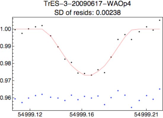
FIG. 1: Wallace 14-inch Telescope Transit: TrES3 The normalized ratio of the light from TrES-3 to several comparison stars is plotted (top points), with a model light curve (solid line). Residuals are plotted below. The standard deviation of the residuals is 0.00238. Exposures were 105 seconds; points shown are 4 binned data points.
The first transit that I observed was a TrES-3 transit. TrES-3 is an excellent planet to observe from Wallace because of its deep transit depth (2.6%) and the large number of good comparison stars within the 18 arcminute field of view of the 14-inch telescopes. On June 16th, my first night out, I had perfect weather and recorded the best data I would get all summer. I used photometry methods in IRAF to reduce the images, and borrowed and edited Elisabeth Adams’ code to reduce the data. I plotted the ratio of light from TrES-3 to various comparison stars and fitted a model curve to this data using Mathematica. This fitted light curve is shown in Figure 1.
I also observed another TrES-3 transit on July 4th which I reduced in the same way as I reduced the first transit. Weather conditions created the additional noise in this light curve when compared to the June 17th TrES-3 transit, and also prevented a flat line after egress from being observed. The light curve is shown in Figure 2.
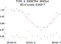
FIG. 2: Wallace 14-inch Telescope Transit: TrES3 The normalized ratio of the light from TrES-3 to several comparison stars is plotted (top points), with a model light curve (solid line). Residuals are plotted below. The standard deviation of the residuals is 0.00317. Exposures were varied between 120 and 240 seconds; points shown are 5 binned data points.
A transit of HAT-P-7b shown in Figure 3. It is a shallow transit; its change in flux is 0.6%. This observation was also taken with a 14-inch telescope at Wallace Observatory. This is a partial transit due to weather conditions that prevented egress from being observable. The noise in this light curve demonstrates one of the big challenges I have faced observing with these smaller telescopes; the 14-inch telescopes are being pushed to their observational limits with shallow transits such as this one. It would be impossible to precisely constrain the time of the transit to within seconds or even to within several minutes.
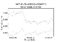
FIG. 3: HAT-P-7b Transit Using 14-inch Telescope The normalized ratio of the light from HAT-P-7 to four comparison stars is plotted (top points), with a model light curve (solid line). Residuals are plotted below. Egress is not plotted because weather prevented the end of the transit from being observed. The standard deviation of the residuals is 0.00124 (10% of the transit depth). Exposures were 60 seconds; points shown are 6 binned data points.
A transit of HAT-P-5b is shown in Figure 4. Weather conditions again prevented egress from being observed.
Figure 5 shows a partial transit of HD17156b. This is a long transit so partial transits are nearly always observed instead of full transits. Note that this transit is problematic; it is not entirely clear that I observe a transit through the noise. The main problem with this light curve is that the star HD17156 is so much brighter than the surrounding stars. In order to avoid saturating the target star, exposures were only 5 seconds long. This meant, however, that counts on comparison stars were very low. If I were to try and observe this transit again, I would shift
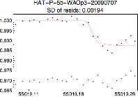
FIG. 4: HAT-P-5b Transit Using 14-inch Telescope The normalized ratio of the light from HAT-P-5 to four comparison stars is plotted (top points), with a model light curve (solid line). Residuals are plotted below. Egress is not plotted because weather prevented the end of the transit from being observed. The standard deviation of the residuals is 0.00194. Exposures were 120 seconds; points shown are 5 binned data points.
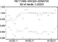
FIG. 5: HD17156b Transit Using 14-inch Telescope The normalized ratio of the light from HD17156 to four comparison stars is plotted (top points), with a model light curve (solid line). Residuals are plotted below. Egress is not plotted because weather prevented the end of the transit from being observed. The standard deviation of the residuals is 0.00233. Exposures were 5 seconds; points shown are 20 binned data points.
my field of view slightly to include some different comparison stars. This is also a very shallow transit (0.5%) which appears to be somewhat out of the range of observation for the Wallace 14-inch telescopes.
In addition, this summer I have spent time
FIG. 6: TrES-1 Transit from IRTF The normalized ratio of the light from TrES-1 to one comparison star is plotted. Exposures were between 1 and 2 seconds. The dotted lines show the mean and standard deviations of the flat part of the light curve
reducing some of Elisabeth Adams’ data from the IRTF telescope in Hawaii. She remotely observed 4 TrES-1 transits over the course of the summer; this data will be used in a transit timing paper. The data reduction is a challenge in part due to the large number of frames, which could be over 10,000 frames per transit; it takes much longer to process than my own data, which usually had between 100 and 1000 frames. I show an example of a TrES-1 transit that I reduced in figure 6.
3. FURTHER WORK FOR SENIOR THESIS
There are several further steps that I will take during the fall semester, since I intend to develop this research experience into a senior thesis project. I will continue to observe and analyze transits; there are several transits that I observed in August for which I am still completing my data reduction. Now that the 24-inch telescope is functioning again at Wallace Observatory, I will attempt to use it in addition to the smaller 14-inch telescopes; I hope that the larger telescope will improve the noise in some of my data since it gathers nearly three times as many photons.
While I plan to write my thesis about extrasolar planet transit observation, I do not yet have a definitive topic and outline for this project. I have learned a lot this summer about observation and data reduction skills. I plan to incorporate both these skills that I have learned as well as the actual data I have collected and reduced this summer for my thesis project during my senior year.
Acknowledgments
I gratefully acknowledge Jim Elliot, Elisabeth Adams, Tim Brothers, Mike Person, Amanda Zangari, Matt Lockhart, and all the other undergraduate observers for supporting this project.